本文主要内容翻译整理自:Easy multi-panel plots in R using facet_wrap() and facet_grid() from ggplot2,部分代码有修改。 ggplot2 一个非常强大的功能就是进行 multi-panel plots 的呈现,也就是我们常说的分面(facet)。通过使用 facet_wrap() 或者 facet_grid() 这样的函数我们就可以很方面的将单一的一个图变为多个相关的图。本文将通过一个具体的数据示例帮助你理解 ggplot2 分面的不同方法以及参数。 为了纪念 Captain Marvel 和即将到来的 Avengers: Endgame ,我们将使用来自 Kaggle 的 漫威角色数据集 我们将主要用到其中的 3 个变量信息: 在进行分析之前,首先对数据进行几步清洗,比如去除上述三个变量存在缺失值的数据,对变量进行更简单的重命名,同时因为涉及到的角色太多我们只选择那些出现次数大于 100 次的角色。 在整篇文章中,我们将生成按年份分组的演员数来作为整个分析过程的开始,在某些情况下还会生成其他一些分组变量。对于这个初始图我们仅是按年进行简单的计算。 首先画一个由线点构成的单一图形。 首先按照 year 和 alignment 来统计数目 只需要在上面绘图命令的结尾加上 这张图拥有了更大的信息量,比如我们可以发现在 1963 和 1964 年出现了大量的坏蛋,随后则逐渐减少;而好人在后面还是一直在稳定的加入。在未特殊指定的情况下,这里 如果对 如果想要排除行或者列变量可以通过 在时间序列数据中,使用两条不同颜色的线有时比分面效率要更高。 颜色和分面混用也不失为一个高效的选择。 在 faceting 函数中,有一些参数是通用的,只是在使用略有差别。 可以使用 本文作者:思考问题的熊 版权声明:本博客所有文章除特别声明外,均采用 知识共享署名 - 非商业性使用 - 禁止演绎 4.0 国际许可协议 (CC BY-NC-ND 4.0) 进行许可。 如果你对这篇文章感兴趣,欢迎通过邮箱订阅我的 「熊言熊语」会员通讯,我将第一时间与你分享肿瘤生物医药领域最新行业研究进展和我的所思所学所想,点此链接即可进行免费订阅。
数据准备集
library(ggplot2)
library(dplyr)

marvel <- readr::read_csv("marvel-wikia-data.csv")

marvel <- filter(marvel, SEX != "", ALIGN !="", Year != "") %>%
  filter(!is.na(APPEARANCES), APPEARANCES>100) %>%
  mutate(SEX = stringr::str_replace(SEX, "Characters", "")) %>%
  arrange(desc(APPEARANCES)) %>%
  rename(gender = SEX) %>%
  rename_all(tolower)
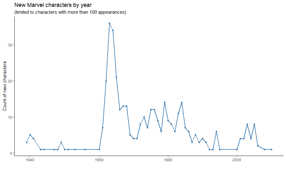
按照年份统计角色出现次数
marvel_count <- count(marvel, year)
glimpse(marvel_count)
# glimpse 可以展示数据的观测和变量数量以及每一列的名字和尽可能多的列信息,和 structure 类似。
## Observations: 57
## Variables: 2
## $ year <dbl> 1939, 1940, 1941, 1943, 1944, 1947, 1948, 1949, 1950, 195...
## $ n    <int> 3, 5, 4, 1, 1, 1, 1, 3, 1, 1, 1, 1, 1, 7, 20, 36, 34, 21,...
ggplot(data = marvel_count, aes(year, n)) +
    geom_line(color = "steelblue",size = 1) +
    geom_point(color="steelblue") +
    theme_classic() +
    labs(title = "New Marvel characters by year",
         subtitle = "(limited to characters with more than 100 appearances)",
         y = "Count of new characters", x = "")
使用 facet_wrap() 按照角色人设分面
marvel_count <- count(marvel, year, align)
glimpse(marvel_count)
## Observations: 114
## Variables: 3
## $ year  <dbl> 1939, 1939, 1940, 1940, 1941, 1941, 1943, 1944, 1947, 19...
## $ align <chr> "Good Characters", "Neutral Characters", "Bad Characters...
## $ n     <int> 2, 1, 1, 4, 1, 3, 1, 1, 1, 1, 3, 1, 1, 1, 1, 1, 1, 6, 4,...
+ facet_wrap(~ align) 就可以绘制按照 alignment 分面的 multi-panel plotggplot(data = marvel_count, aes(year, n)) +
geom_line(color = "steelblue",size = 1) +
geom_point(color="steelblue") +
theme_classic() +
labs(title = "New Marvel characters by year",
subtitle = "(limited to characters with more than 100 appearances)",
y = "Count of new characters", x = "") +
facet_wrap(~ align)
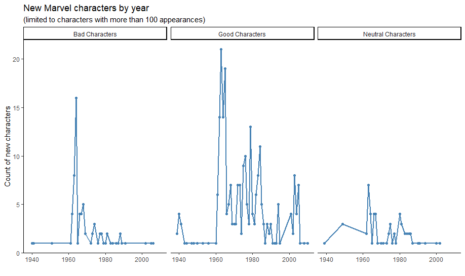
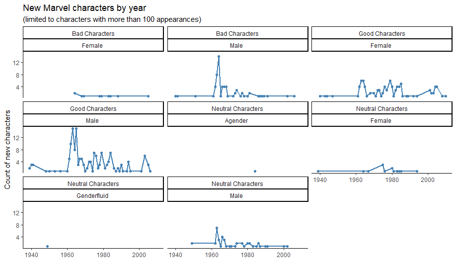
facet_wrap 选择了一行展示三个图。facet_wrap() 使用两个变量,其实只需要简单的使用 + 来进行链接。但是通常情况下,为了更好的调整布局,建议使用 facet_grid()。marvel_count <- count(marvel, year, align, gender)
ggplot(data = marvel_count, aes(year, n)) +
geom_line(color = "steelblue",size = 1) +
geom_point(color="steelblue") +
theme_classic() +
labs(title = "New Marvel characters by year",
subtitle = "(limited to characters with more than 100 appearances)",
y = "Count of new characters", x = "") +
facet_wrap(~ align + gender)
按照 facet_grid() 指定行列进行绘图
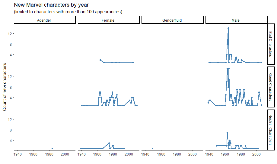
facet_grid(row_variable ~ column_variable) 可以通过指定行和列来进行绘图,例如使用 align 作为行变量,gender 作为列变量ggplot(data = marvel_count, aes(year, n)) +
geom_line(color = "steelblue",size = 1) +
geom_point(color="steelblue") +
theme_classic() +
labs(title = "New Marvel characters by year",
subtitle = "(limited to characters with more than 100 appearances)",
y = "Count of new characters", x = "") +
facet_grid(align ~ gender)
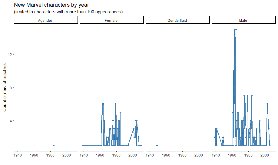
. 来进行代替。如下所示:ggplot(data = marvel_count, aes(year, n)) +
geom_line(color = "steelblue",size = 1) +
geom_point(color="steelblue") +
theme_classic() +
labs(title = "New Marvel characters by year",
subtitle = "(limited to characters with more than 100 appearances)",
y = "Count of new characters", x = "") +
facet_grid(. ~ gender)
ggplot(data = marvel_count, aes(year, n)) +
geom_line(color = "steelblue",size = 1) +
geom_point(color="steelblue") +
theme_classic() +
labs(title = "New Marvel characters by year",
subtitle = "(limited to characters with more than 100 appearances)",
y = "Count of new characters", x = "") +
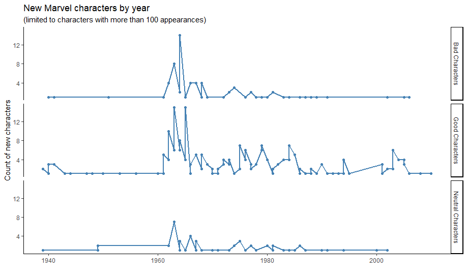
facet_grid(align ~ .)
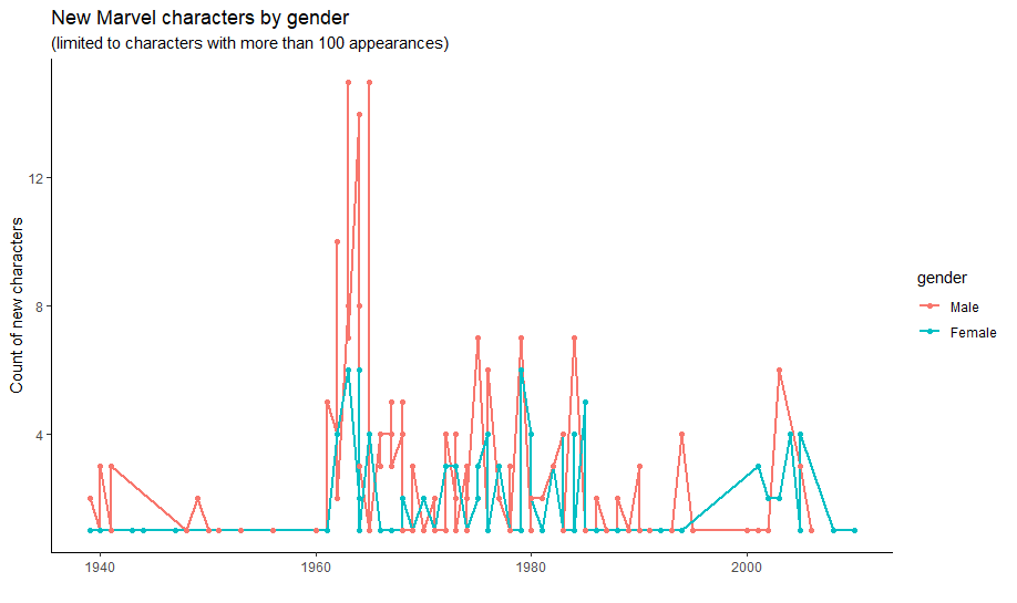
颜色有时效果更好
# Limit to male and female and change levels for drawing order
marvel_count <- filter(marvel_count, gender%in%c("Female", "Male")) %>%
    mutate(gender = factor(gender, levels = c("Male", "Female")))

ggplot(data = marvel_count, aes(year, n, color = gender)) +
    geom_line(size = 1) +
    geom_point() +
    theme_classic() +
    labs(title = "New Marvel characters by gender",
         subtitle = "(limited to characters with more than 100 appearances)",
         y = "Count of new characters", x = "")
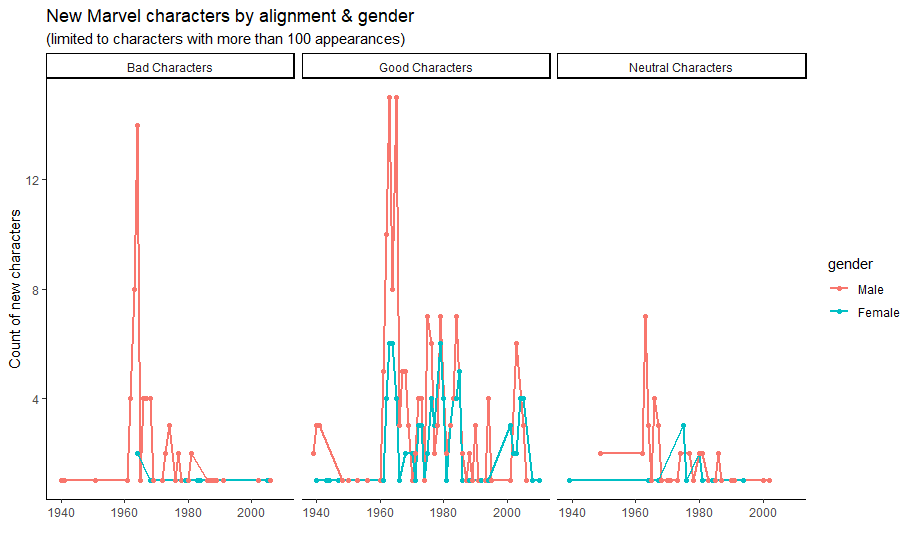
ggplot(data = marvel_count, aes(year, n, color = gender)) +
    geom_line(size = 1) +
    geom_point() +
    theme_classic() +
    labs(title = "New Marvel characters by alignment & gender",
         subtitle = "(limited to characters with more than 100 appearances)",
         y = "Count of new characters", x = "")+
    facet_grid(. ~ align)
几个常用参数
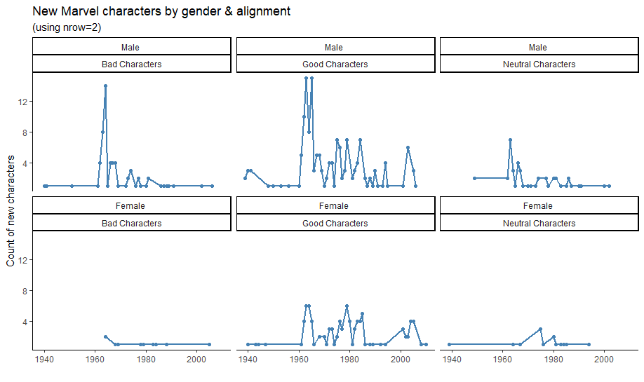
nrow 或者 ncol
facet_wrap() 有效ggplot(data = marvel_count, aes(year, n)) +
geom_line(color = "steelblue",size = 1) +
geom_point(color = "steelblue") +
theme_classic() +
facet_wrap(~ gender + align, nrow = 2) +
labs(title = "New Marvel characters by gender & alignment",
subtitle = "(using nrow=2)",
y = "Count of new characters", x = "")
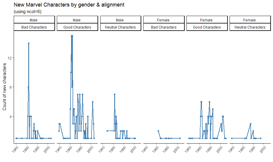
ggplot(data = marvel_count, aes(year, n)) +
  geom_line(color = "steelblue", size = 1) +
  geom_point(color ="steelblue") +
  theme_classic() +
  facet_wrap(~ gender + align, ncol = 6) +
  labs(title = "New Marvel Characters by gender & alignment",
       subtitle = "(using ncol=6)",
       y = "Count of new characters", x = "") +
  theme(
       axis.text.x = element_text(angle=50, hjust=1)
  )
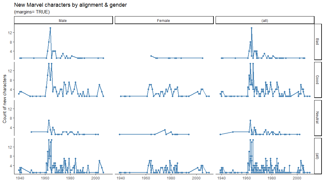
margins
facet_grid 有效marvel_count <-
mutate(marvel_count, align = stringr::str_replace(align, "Characters", ""))
ggplot(data = marvel_count, aes(year, n)) +
geom_line(color = "steelblue", size = 1) +
geom_point(color = "steelblue") +
theme_classic() +
labs(title = "New Marvel characters by alignment & gender",
subtitle = "(margins= TRUE)",
y = "Count of new characters", x = "") +
facet_grid(align ~ gender, margins=TRUE)
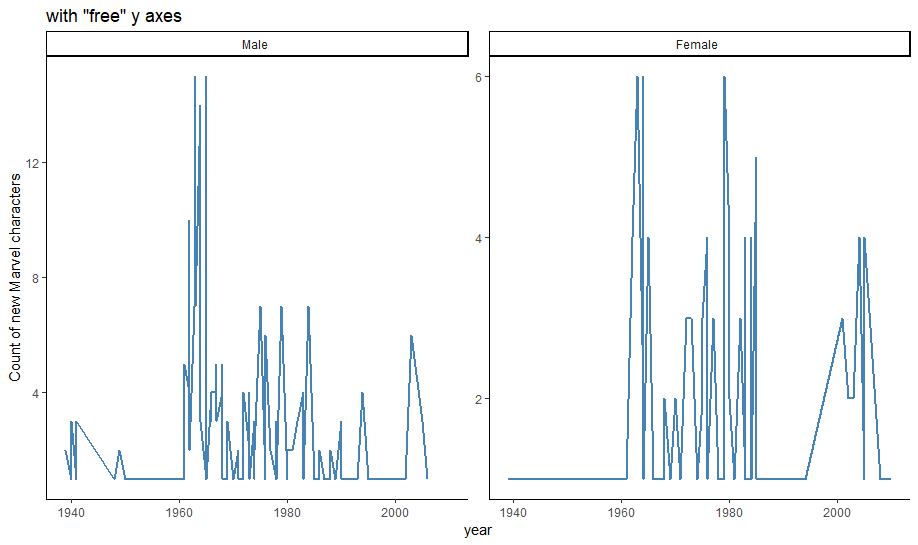
自由定义不一致的 Y 轴
scales = "free" 或者 scales = "free_x" 或者 "free_y" 进行设置。但是一定要注意这样的图可能会使读者造成误解。ggplot(marvel_count, aes(year, n)) +
geom_line(color = "steelblue", size = 1) +
facet_wrap(~gender, scales = "free_y")+
theme_classic() +
labs(title = 'with"free"y axes' ,
y = "Count of new Marvel characters")
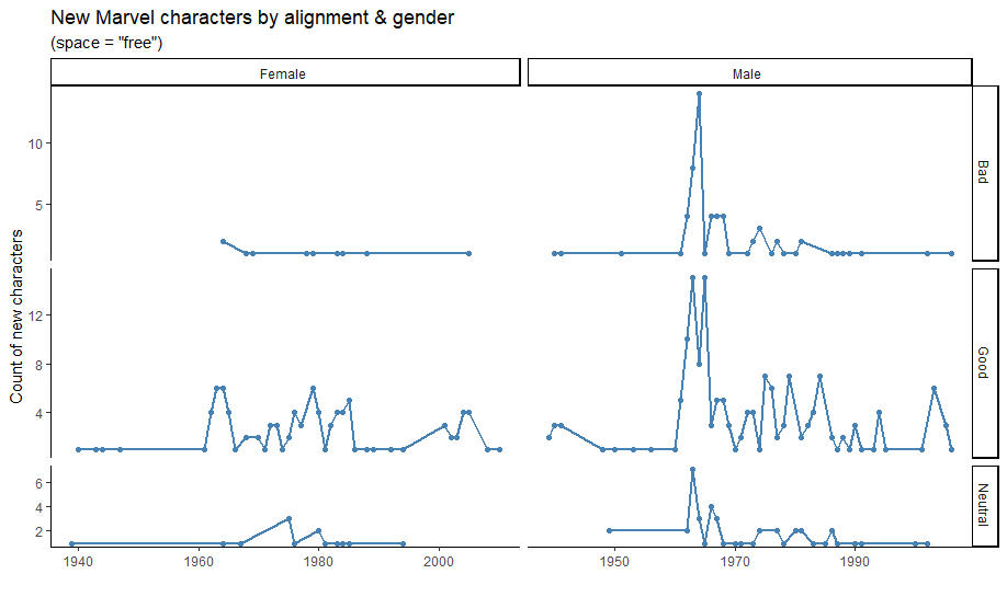
space
facet_grid() 有效scales = "free" 一起连用ggplot(data = marvel_count, aes(year, n)) +
geom_line(color = "steelblue", size = 1) +
geom_point(color = "steelblue") +
theme_classic() +
labs(title = "New Marvel characters by alignment & gender",
subtitle = '(space ="free")',
y = "Count of new characters", x = "") +
facet_grid(align ~ gender, space="free", scales="free")
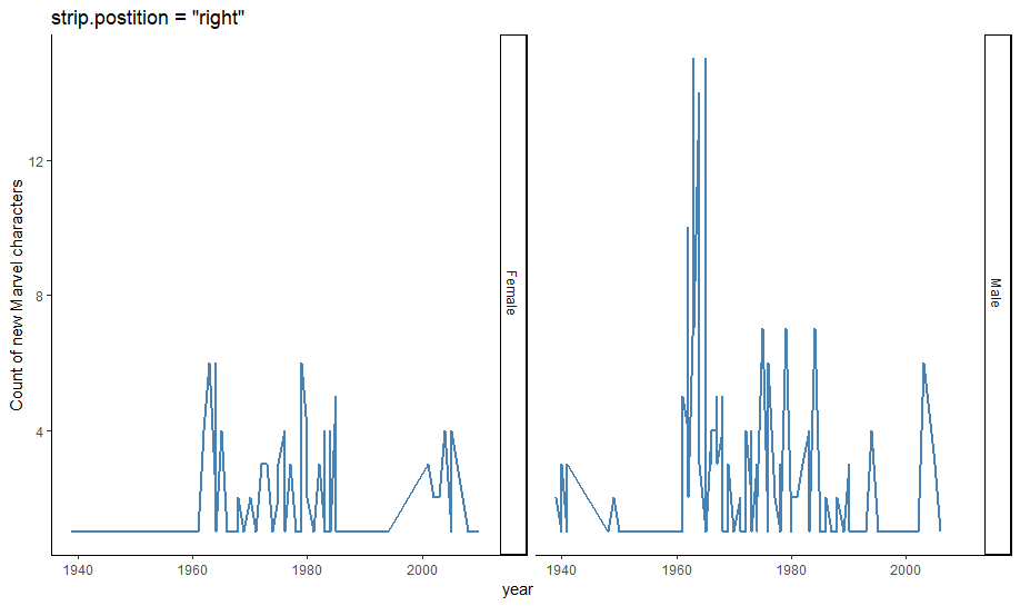
strip.position
facet_wrap() 可用ggplot(marvel_count, aes(year, n)) +
geom_line(color = "steelblue", size = 1) +
theme_classic() +
facet_wrap(~gender, strip.position = "right") +
labs(title = 'strip.postition ="right"',
y = "Count of new Marvel characters")
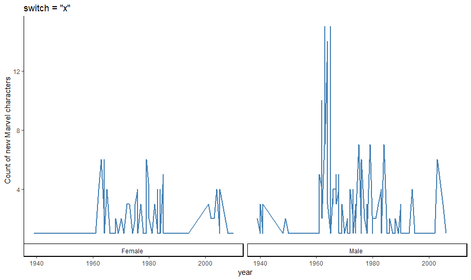
switch
facet_grid() 有效x 会让 label 在底部,y 右改为左,both 则改为左下ggplot(marvel_count, aes(year, n)) +
geom_line(color = "Steelblue", size = 1) +
theme_classic() +
facet_grid(~gender, switch = "x" ) +
labs(title = 'switch ="x"',
y = "Count of new Marvel characters")
· 分享链接 https://kaopubear.top/blog/2019-04-04-facet-ggplot2/